
Felix Thoemmes


A recurring discussion on Twitter and other social media is whether one should or should not check baseline covariates for balance in a randomized experiment. The discussion comes in various flavors, sometimes focusing on whether the very act of balance checks are meaningful, or whether randomization actually is or is not expected to yield balance, and whether something should or should not be done about unbalanced covariates. Stephen Senn has written a paper on this called “Seven myths of randomisation in clinical trials” (http://onlinelibrary.wiley.com/doi/10.1002/sim.5713/pdf). I highly recommend reading it. There is also an interesting blog post by John Myles White (http://www.johnmyleswhite.com/notebook/2017/04/06/covariate-based-diagnostics-for-randomized-experiments-are-often-misleading/) that argues that we typically should not check for balance. Here is a brief excerpt:
“balancing covariates is neither necessary nor sufficient for an experiment’s inferences to be accurate. […] the lesson from this example is simple: we must not go looking for imbalances, because we will always be able to find them.”
In this blog post, I will try to make an argument that balance checks in randomized experiment can be a good thing.
I would like to illustrate my point with a little anecdote. A couple of years ago, I participated in a study in Nutritional Sciences here at Cornell. The study looked at ways that people can lose weight (more precisely, maintain weight over time.) After seeing a flyer on a billboard, I signed up for the study via email, I was assigned a participant number, and then I was summoned for an intital interview a few days later. Upon my arrivial I was greeted by an undergrad student who was seated at a table with a laptop in front of her. She had a list with participants printed out next to her, and I believe she was copying names of participants into an Excel sheet on her laptop. Next to her were two neatly arranged piles of instructions - as I later learned one for the control and one for the treatment group. She took my name, consulted the Excel sheet, and then handed me the instruction sheet for the treatment group. After that I was ushered to the next room to be measured, weighted, and tested by another undergrad student. Even though I don’t know for sure, but I assume that the Excel sheet contained random numbers that coded assignment to either treatment or control group, and that my name, and my participant number, were somehow linked to the random numbers, and thus the random assignment to one of the treatment arms. Overall, I believe this is a sensible way to randomly assign participants to conditions.
But let’s imagine that this scenario played out a little differently. Let’s imagine that the undergrad happened to like this particular treatment for not gaining weight. Maybe she learned about it during lab meetings, and she really believes that it’s a great treatment. Now she sits there with her laptop, and randomly assigns participants to these conditions. But then a person comes to her, she sees that the person may be overweight, and she thinks to herself “Wouldn’t it be great if that person was randomly assigned to the treatment”? Unluckily, the random number generator assigned that person to the control group, but at this point it becomes really easy to change that assignment in the Excel sheet - and so the person ends up in the treatment group - contrary to the actual random assignment. The next time that a participant comes in who doesn’t look like he or she would need the treatment, the student reverses another assignment to balance the number of participants. And so it continues… Just to clarify, I have no reason whatsoever that this happened in this particular trial - I am just using it as an example.
The result of this is that the randomization is compromised. Instead of being randomly assigned, participants are now assigned based on the subjective belief of an undergrad as to who might experience the greatest benefit from the treatment. And if we further believe that the undergrad assigned those individuals that looked overweight to the treatment, we will clearly see that participants in the treatment condition weight more than participants in the control condition, prior to treatment. We thus have covariate imbalance. And unfortunately, the covariate ‘intital weight’ is most likely also related to our outcome of interest, which presumambly is weight loss over a period of time.
You might argue that such blatant disregard for the randomization is rare, and I might agree. Further, if done with intention, you might think it is even unethical, and I’d agree even more. But if it were to happen, how would one know? The answer is, by checking the balance of the covariates at baseline. In a randomized experiment in which randomization was not compromised, we should not expect to see these types of imbalances often. They still can happen by chance - in fact, we know what this chance level is, a-priori. But in an experiment with compromised randomization we should expect to see these imbalances routinely - precisely on those variables that were used to determine treatment. For me, this implies that we should check balance on those covariates that we believe could have been used to improperly compromise the randomization. Hopefully, we have some expert knowledge of what those variables could be. In the example that I have given, initial weight at baseline seems like a good candidate.
Let’s demonstrate the intuition that I outlined in the anecdote above quickly using a simulation. We consider again a randomized trial for a weight loss intervention. The outcome of interest is weight three month post-test. In our simulation we consider that there are 5 pre-test covariates (one of them initial weight). The covariates themselves are for simplicity uncorrelated, and they have varying relationships to the outcome (weight at post-test), ranging from positive (intital weight) to negative, including zero. In the proper randomized experiment, the treatment is determined by a fair coin flip. The effect of the treatment varies as a function of initial weight (individuals with low weight don’t benefit from the treatment at all, whereas individuals with higher weights, benefit from the treatment, but the average effect is a weight loss of 3000 grams (3kg). The effect modification is modeled via an interaction term between treatment and intital weight (the treatment is more effective by .2kg for every increase of 10kg in weight).
To get an idea of what we would expect in a properly conducted randomized trial, we simulate 10,000 RCTs with a fixed sample size of 200, and proper randomization.
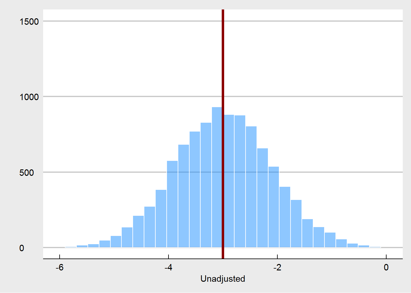
We see that the true treatment effect is (of course) recovered without bias.
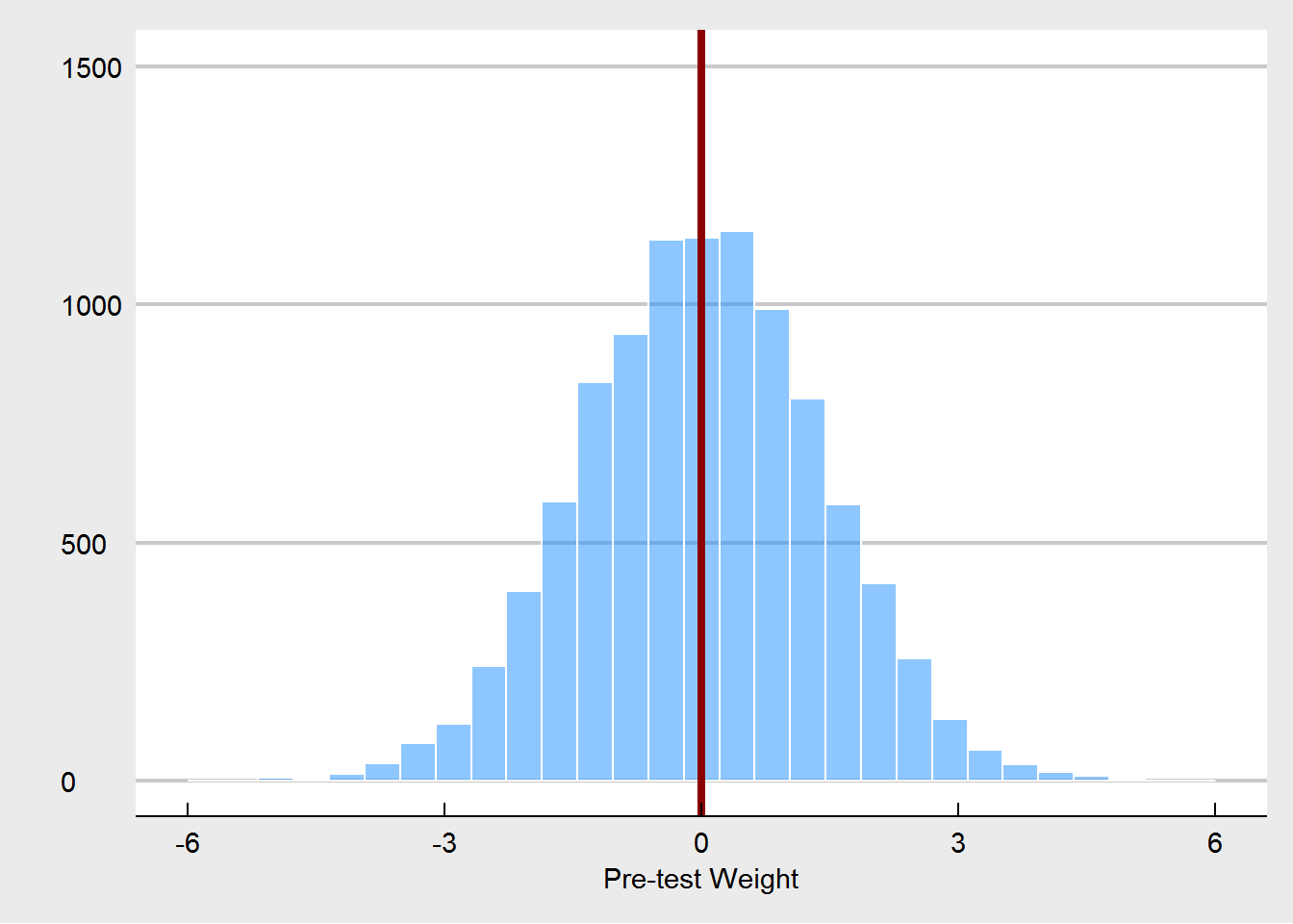
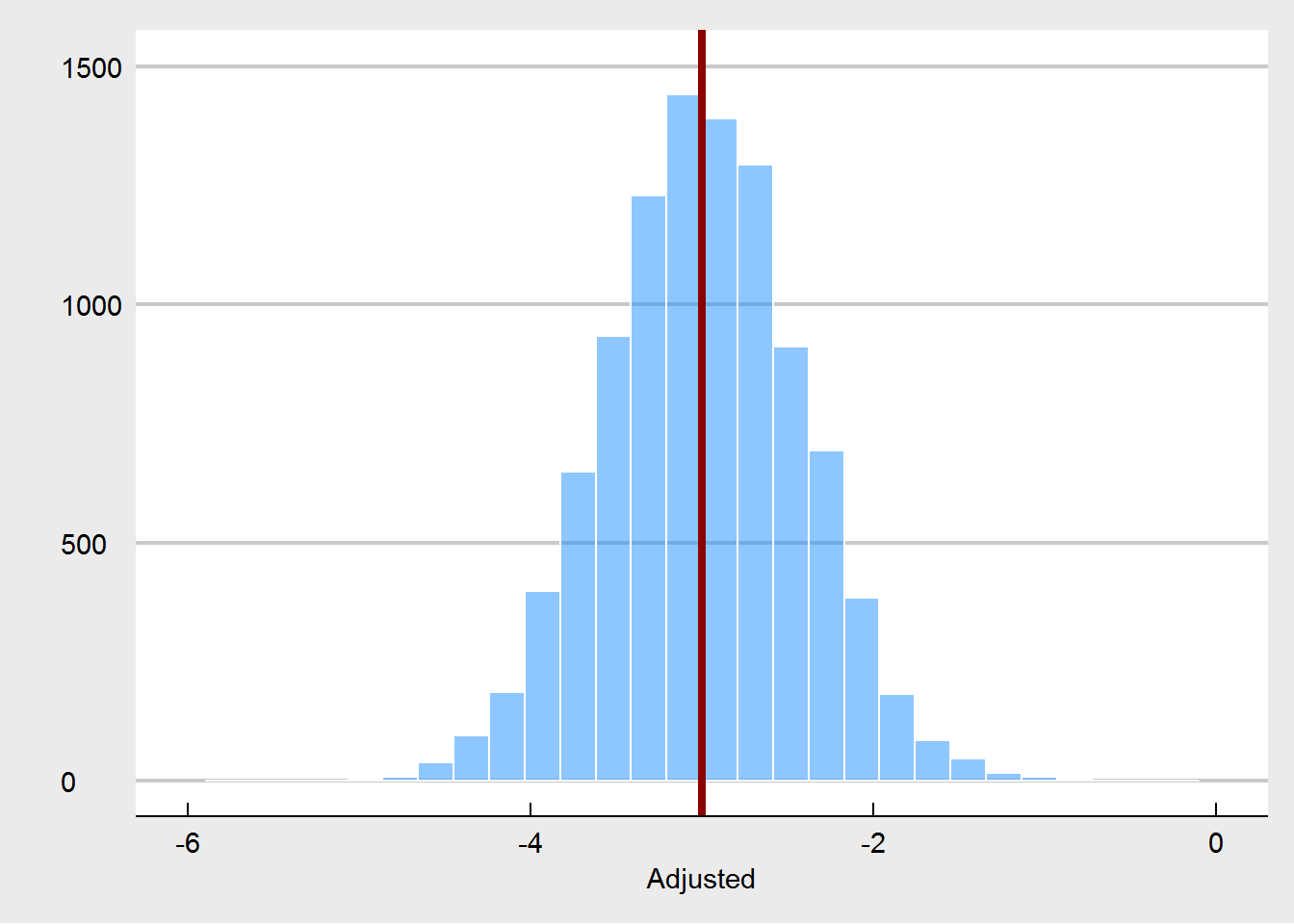
We also see that on occasion pre-treatment weights are imbalanced. In a properly randomized experiment, that’s OK, as these imbalances are often offset by other imbalances over a wide range of potential covariates. They do not harm our inference, as explained by Senn (2013). Also as expected, using pre-test weight as a covariate also yields an unbiased estimator, and it increases precision.
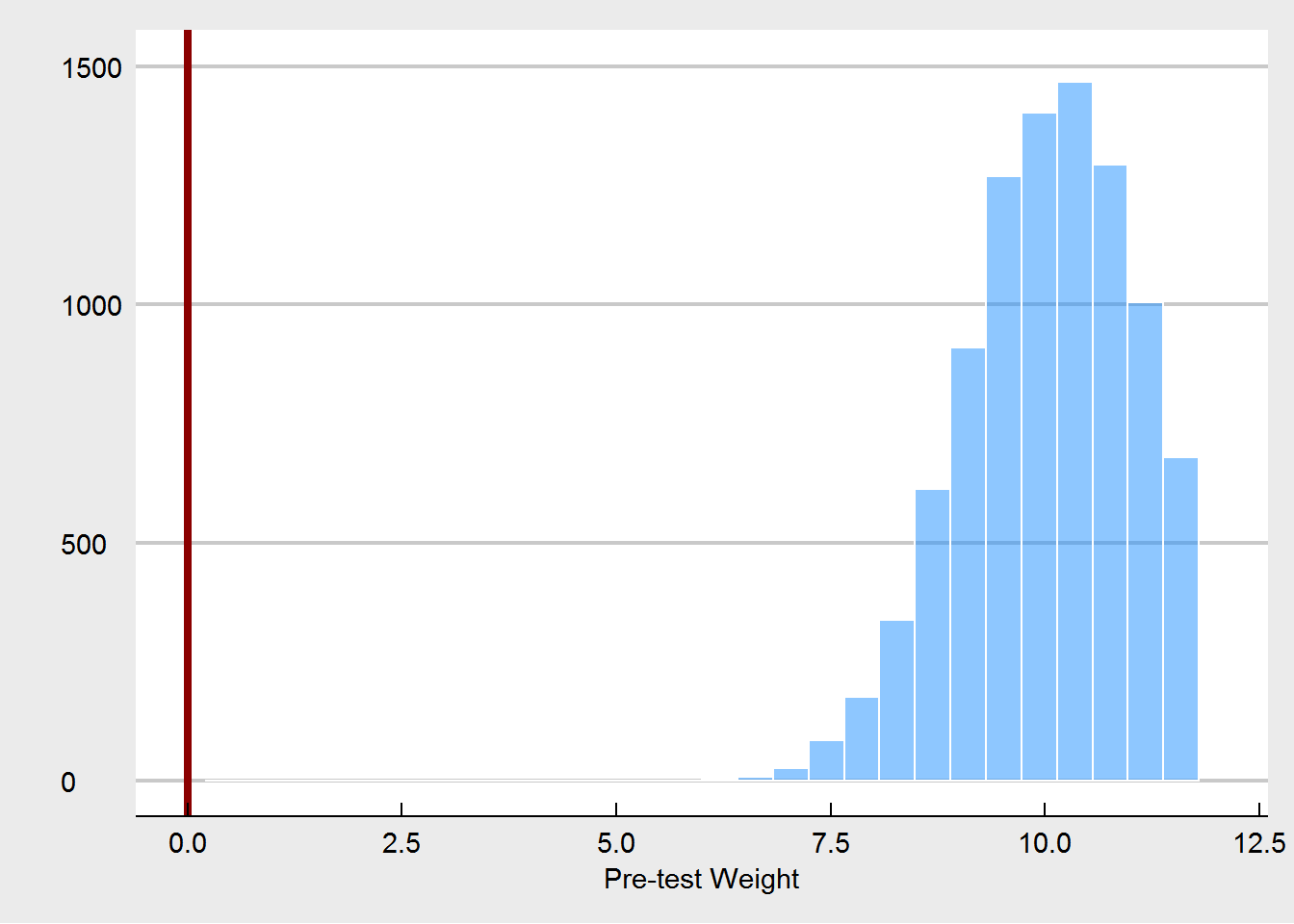
Let’s turn to the experiment in which randomization is compromised. We consider that randomization was compromised in the following manner: if participants were in the highest quartile of weight at pre-test, the probability for them to be assigned to the treatment condition changed from 50% (fair coin flip) to 90%. Likewise, the lowest quartile of weight had only a probabilty of 10% to be assigned to the treatment. This crudely models a behavior of somebody who is tweaking the randomization as to steer people who might benefit most from the treatment towards the treatment, but in order to maintain balance, steers other people who are less likely to benefit away from the treatment. We would expect that such a non-random assignment, would yield larger treatment effects at post-test.
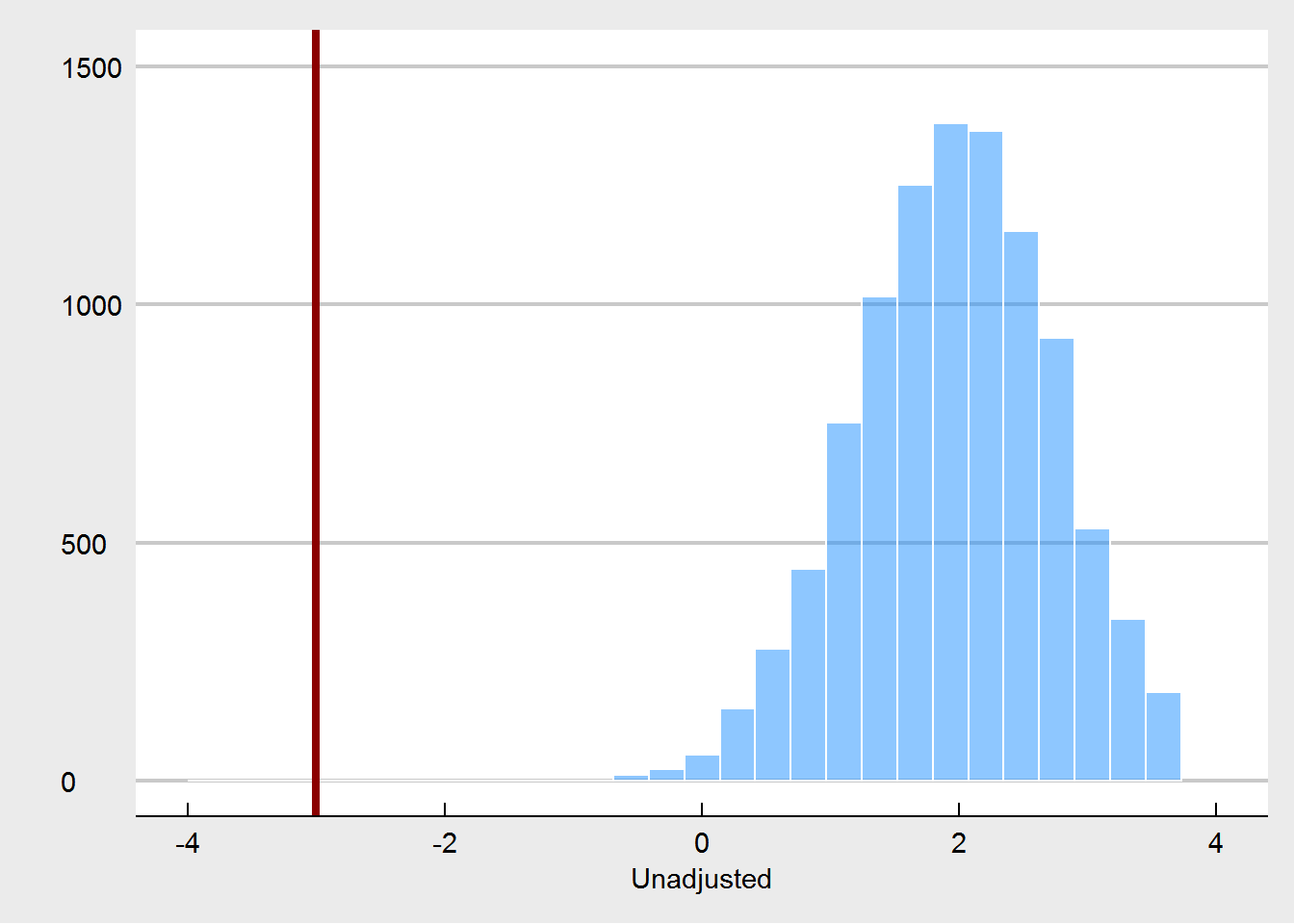
What we see here, is that the unadjusted treatment effect is now a biased estimator of the true treatment effect. The treatment effect is estimated to be way too high. Using pre-test weight as a covariate fixes this, as expected. But we are also seeing that pre-test weights are much more unbalanced, especially in comparison to the random imbalances that emerged under the proper randomization.

None of this is really new - in fact these kind of simulations have been done many times before. I think the critical point is that when people say that covariate imbalances are not important, they are assuming properly conducted randomization. If this is in fact the case, then it is true that these imbalances are just Type I errors, random chance, and do not harm our inference. But if the randomization is compromised, then one possible way to spot this is to see unusual imbalances at pre-test. And that is why we should care about them.
In the recent paper by Deaton and Cartwrith (http://www.nber.org/papers/w22595.pdf), the authors write: “These tests [and they are referring to balance tests of pre-treatment variables in randomized trials] are appropriate for unbiasedness if we are concerned that the random number generator might have failed, or if we are worried that the randomization is undermined by non-blinded subjects who systematically undermine the allocation.” I typically would put much faith in usual random number generators in R or other software, but depending on the particular trial, I would be more worried about undermining of the actual randomization.
In summary, when you are conducting and reporting balance tests, you are testing whether your randomization was compromised by factors that are independent of the generation of the random numbers. By showing others that such compromised randomization did likely not happen, you increase the confidence that others can have in the results of your ranomized study.
UPDATE (6/13/18): The blog post triggered interesting discussions with Tim van der Zee, Frank Harrell, and Jeffrey Blume. Tim, and Frank objected, saying that an observed imbalance could only with great difficulty be categorized as either emerging from random imbalance, or due to cheating (compromised randomization). They expressed concerns that post-hoc balance checking and adjustment can lead to irreproducible results. One point of agreement is that it is preferable to also have procedural information about the randomization. Imbalance in addition to procedural information that suggests possible cheating makes for a much stronger case than only seeing imbalance. Another strong point of agreement with Frank is that, I too, endorse defining important covariates a-priori (essentially pre-register which covariates you think are important to be balanced). Jeffrey Blume suggested that imbalances should not be ignored post-randomization, and referred to doing this as “randomize, and close your eyes”. I discussed this further with some colleagues over in econ, and would like to highlight one point that they made: when we evaluate randomization in simulations studies (like I did in the blog post), we tend to forget that in the real world, randomization is a process that is typically (at some stage of the experiment) executed by humans. Humans are fallible, and therefore randomization is too. We should (and can) design randomization studies so that we minimize the chance that the randomization procedure is compromised. If we don’t design them this way, and suspect cheating, we can check balance.
#true experiment
set.seed(1234)
preweight <- rnorm(200,80,10)
cov2 <- rnorm(200,0,1)
cov3 <- rnorm(200,0,1)
cov4 <- rnorm(200,0,1)
cov5 <- rnorm(200,0,1)
treat <- rbinom(200,1,.5)
postweight <- 40 + .5*preweight - 2.4*treat - .2*I(treat*preweight/10) + .2*cov2 - .6*cov3 - .3*cov4 + rnorm(200,0,8)

df1 <- data.frame(preweight,cov2,cov3,cov4,cov5,postweight,treat)

library(tidyr)
library(ggplot2)
library(viridis)
library(ggthemes)
df2 <- data.frame(cbind(c(preweight,postweight),factor(rep(1:2,each=200)),factor(rep(1:200,times=2)),factor(c(treat,treat))))
names(df2) <- c("Weight","Time","id","Treatment")
df2$Time <- factor(df2$Time)
df2$id <- factor(df2$id)
df2$Treatment <- factor(df2$Treatment)
levels(df2$Treatment) <- c("Control","Treatment")
levels(df2$Time) <- c("Pre","Post")
ggplot(df2,aes(x=Time,y=Weight,group=id,col=Treatment)) + geom_point(alpha=.5) + geom_line(alpha=.3) +
  theme_economist_white() + scale_color_viridis(option = "plasma",discrete = TRUE,alpha=.3,begin=0,end=.6)


trueexp <- function() {
  preweight <- rnorm(200,80,10)
  cov2 <- rnorm(200,0,1)
  cov3 <- rnorm(200,0,1)
  cov4 <- rnorm(200,0,1)
  cov5 <- rnorm(200,0,1)
  treat <- rbinom(200,1,.5)
  postweight <- 40 + .5*preweight - 1.4*treat - .2*I(treat*preweight/10) + .2*cov2 - .6*cov3 - .3*cov4 + rnorm(200,0,4)
  unadj <- lm(postweight~treat)$coef[2]
  adj <- lm(postweight~treat + preweight + I(treat*(scale(preweight,center = TRUE, scale = FALSE))))$coef[2]
  preweightd <- lm(preweight~treat)$coef[2]
  return(c(unadj,adj,preweightd))
}

res1 <- data.frame(t(replicate(10000,trueexp())))
names(res1) <- c("unadj","adj","preweightd")

ggplot(res1,aes(x=unadj)) + geom_histogram(color="white",fill="dodgerblue",alpha=.5) + theme_economist_white() +
  scale_x_continuous(name = "Unadjusted",limits = c(-6,0)) + geom_vline(xintercept = -3,col="darkred",size=1.5) +
  scale_y_continuous(name="", limits=c(0,1500))

ggplot(res1,aes(x=adj)) + geom_histogram(color="white",fill="dodgerblue",alpha=.5) + theme_economist_white() +
  scale_x_continuous(name = "Adjusted",limits=c(-6,0)) + geom_vline(xintercept = -3,col="darkred",size=1.5) +
  scale_y_continuous(name="", limits=c(0,1500))

ggplot(res1,aes(x=preweightd)) + geom_histogram(color="white",fill="dodgerblue",alpha=.5) + theme_economist_white() +
  scale_x_continuous(name = "Pre-test Weight",limits=c(-6,6)) + geom_vline(xintercept = 0,col="darkred",size=1.5) +
  scale_y_continuous(name="", limits=c(0,1500))

ggplot(res1,aes(x=preweightd,y=unadj)) + geom_point(alpha=.2,col="dodgerblue") + theme_economist_white() +
  scale_x_continuous(name="Pre-test differences weight") + scale_y_continuous(name="Unadjusted effect")

ggplot(res1,aes(x=preweightd,y=adj)) + geom_point(alpha=.2,col="dodgerblue") + theme_economist_white() +
  scale_x_continuous(name="Pre-test differences weight") + scale_y_continuous(name="Adjusted effect")


badexp <- function() {
  preweight <- rnorm(200,80,10)
  cov2 <- rnorm(200,0,1)
  cov3 <- rnorm(200,0,1)
  cov4 <- rnorm(200,0,1)
  cov5 <- rnorm(200,0,1)
  treat <- ifelse(preweight > quantile(preweight,.75), rbinom(100,1,.9), ifelse(preweight < quantile(preweight,.25),rbinom(100,1,.1),rbinom(100,1,.5)))
  postweight <- 40 + .5*preweight - 1.4*treat - .2*I(treat*preweight/10) + .2*cov2 - .6*cov3 - .3*cov4 + rnorm(200,0,4)
  unadj <- lm(postweight~treat)$coef[2]
  adj <- lm(postweight~treat + preweight + I(treat*(scale(preweight,center = TRUE, scale = FALSE))))$coef[2]
  preweightd <- lm(preweight~treat)$coef[2]
  return(c(unadj,adj,preweightd))
}


res2 <- data.frame(t(replicate(10000,badexp())))

names(res2) <- c("unadj","adj","preweightd")


ggplot(res2,aes(x=unadj)) + geom_histogram(color="white",fill="dodgerblue",alpha=.5) + theme_economist_white() +
  scale_x_continuous(name = "Unadjusted",limits = c(-4,4)) + geom_vline(xintercept = -3,col="darkred",size=1.5) +
  scale_y_continuous(name="", limits=c(0,1500))

ggplot(res2,aes(x=adj)) + geom_histogram(color="white",fill="dodgerblue",alpha=.5) + theme_economist_white() +
  scale_x_continuous(name = "Adjusted",limits=c(-6,0)) + geom_vline(xintercept = -3,col="darkred",size=1.5) +
  scale_y_continuous(name="", limits=c(0,1500))

ggplot(res2,aes(x=preweightd)) + geom_histogram(color="white",fill="dodgerblue",alpha=.5) + theme_economist_white() +
  scale_x_continuous(name = "Pre-test Weight",limits=c(0,12)) + geom_vline(xintercept = 0,col="darkred",size=1.5) +
  scale_y_continuous(name="", limits=c(0,1500))

ggplot(res2,aes(x=preweightd,y=unadj)) + geom_point(alpha=.2,col="dodgerblue") + theme_economist_white() +
  scale_x_continuous(name="Pre-test differences weight") + scale_y_continuous(name="Unadjusted effect")

ggplot(res2,aes(x=preweightd,y=adj)) + geom_point(alpha=.2,col="dodgerblue") + theme_economist_white() +
  scale_x_continuous(name="Pre-test differences weight") + scale_y_continuous(name="Adjusted effect")