
Felix Thoemmes


About ten years ago I bought myself a set of non-transitive dice. I have occasionally used them in class, but I am afraid that I am more excited about these dice than the average student. The main idea behind non-transitive dice is that out of a set of dice (and under repeated rolls), one die (A) will on average show a higher value than another die (B), and therefore beat it in a game in which the highest roll wins, but at the same time this winning die (A) will be dominated by another die (C), which itself loses to the loser of the first competition (B). If this sounds complicated, just think of rock-paper-scissors, but with dice.
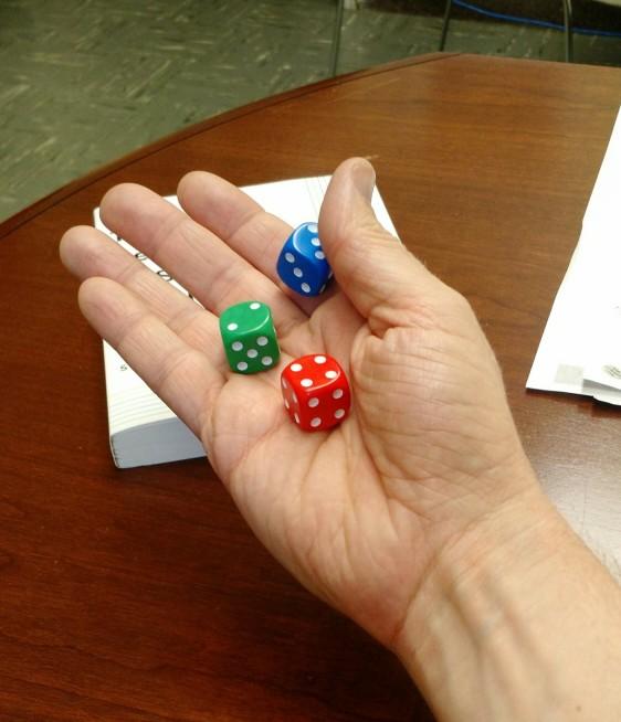
A picture of my non-transitive dice
This particular set of dice has a blue, green, and red die. The blue one has all 3s on it, and one 6. The red one is all 4s, but has one 1, and the green one is an even mix of 2s and 5s. They all have the exact same expected value, which is 3.5. Rolling them in R (code at the end of this post) a couple of thousands of times results in the following, obvious distributions for each die.
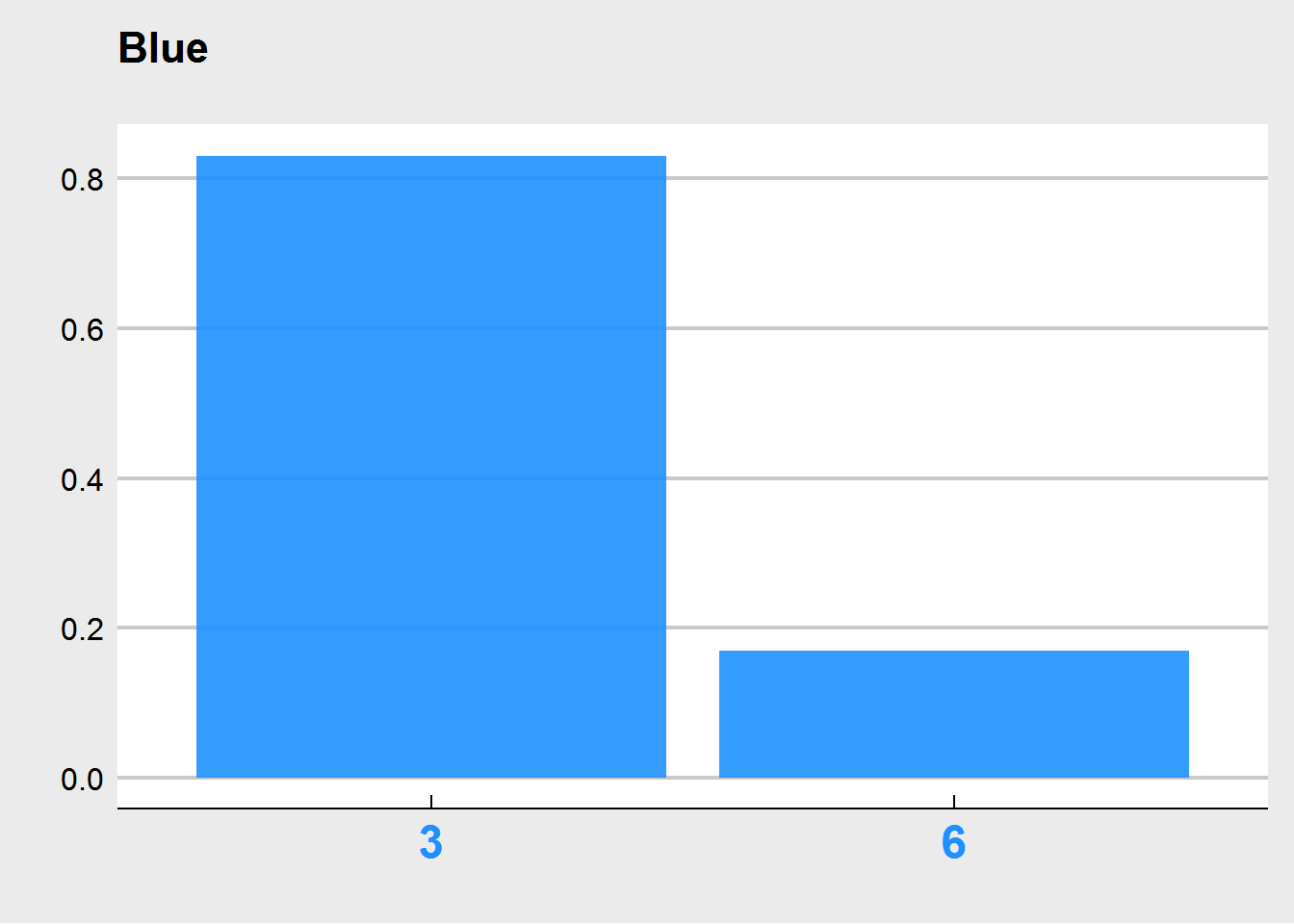
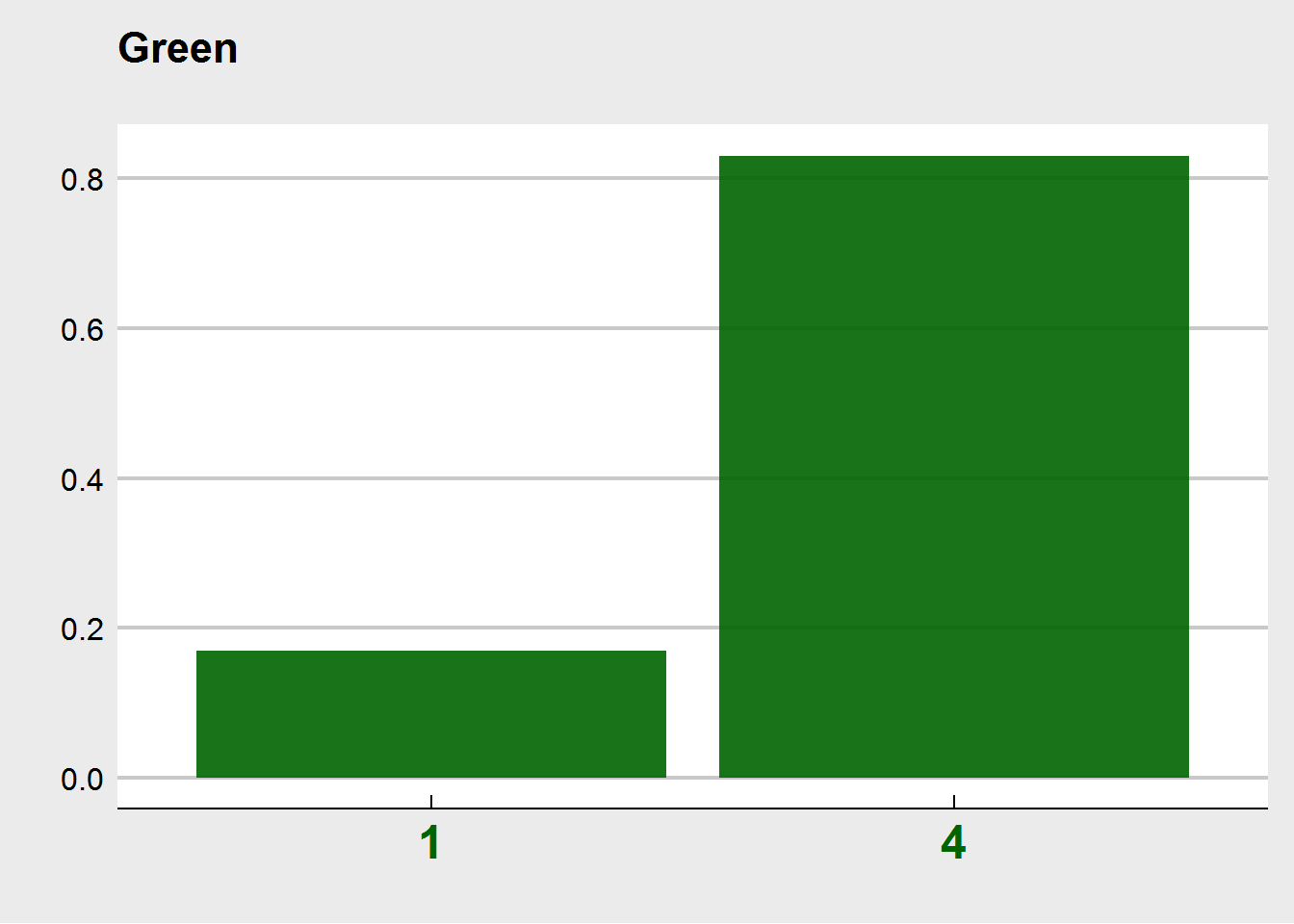
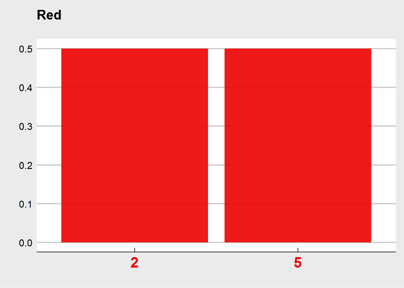
For something simple like this, we didn’t really need to simulate. We can easily see that the e.g., the blue die will have probabilities of \(5/6\) and \(1/6\) to come up 3, or 6, respectively.
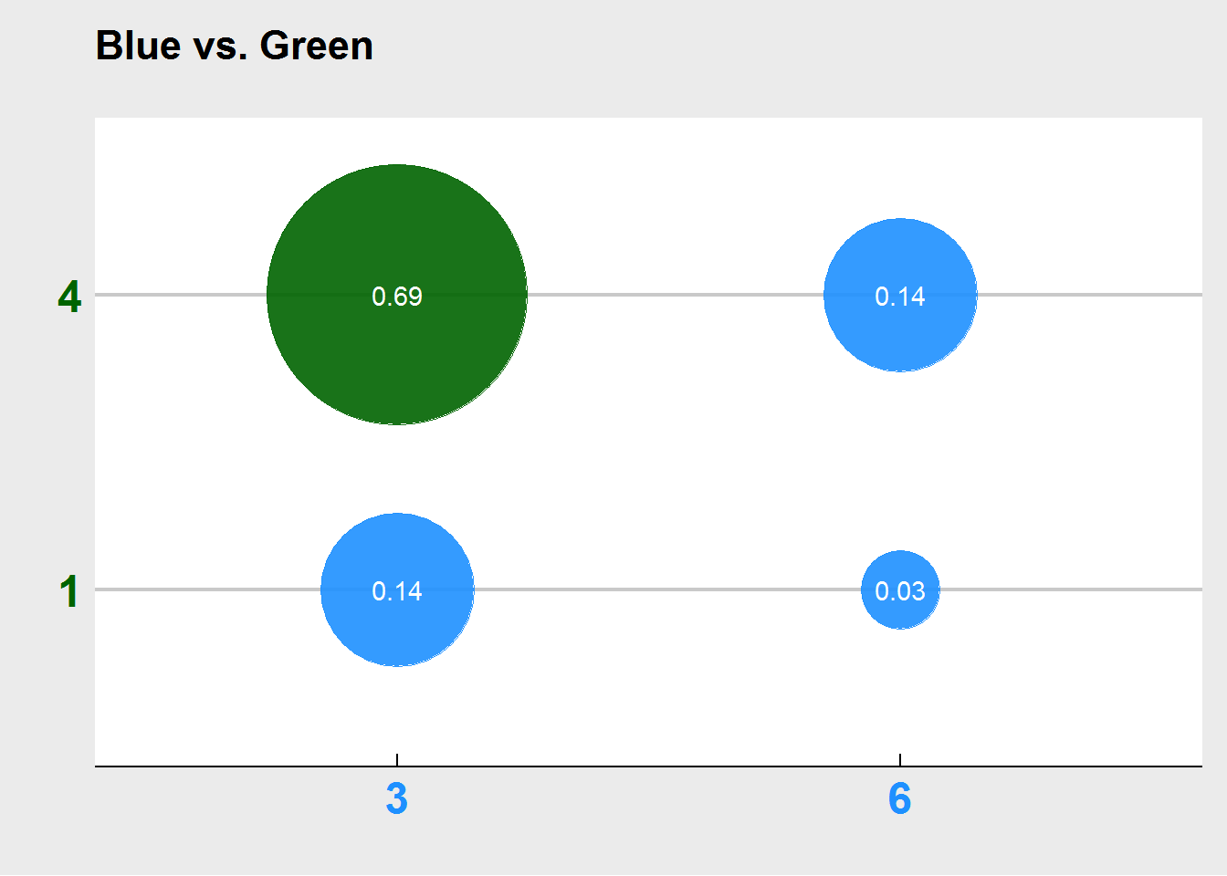
The interesting part now becomes when we consider two dices thrown at the same time. Let’s consider first the blue and the green one. There are only four possible outcomes, the blue one comes up 3, and the green up comes up either 1 or 4, or the blue one comes up 6, and the green one comes up again either 1 or 4. Each of these joint probabilities can be derived easily, because the throws of the different dice are independent. For example, the probability of blue being 3 and green being 4 is \(5/6^2\), so approximately 69%. The plot below shows probabilties of the four possible outcomes, and also color-codes the winner of each constellation. We can clearly see that the green die has a tremendous edge over the blue one. So if faced with the choice of either picking the blue or the green die, you would want to go with the green one.
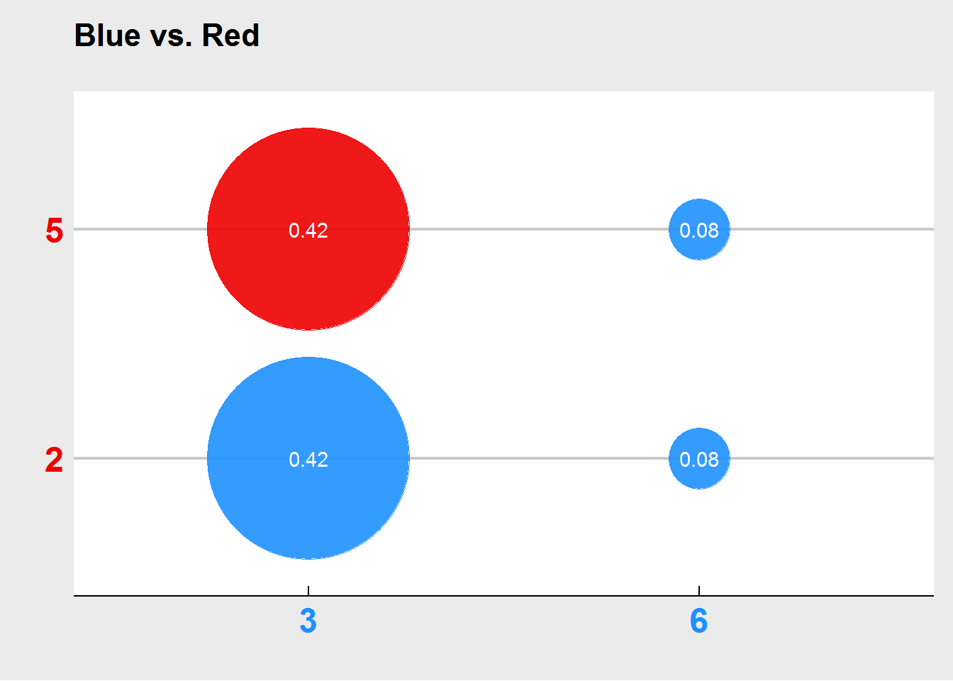
But how does the (previously) losing blue die fare against the red? Let’s repeat this exercise, and have a look at the plot below. Now we find that the blue one has a slight edge against the red one. It’s not as extreme as in the previous case, but it’s there, and in the long run, you would win with the blue die over the red one. At this point we may think that the green die is the best, followed by the blue, and the red one is the worst.
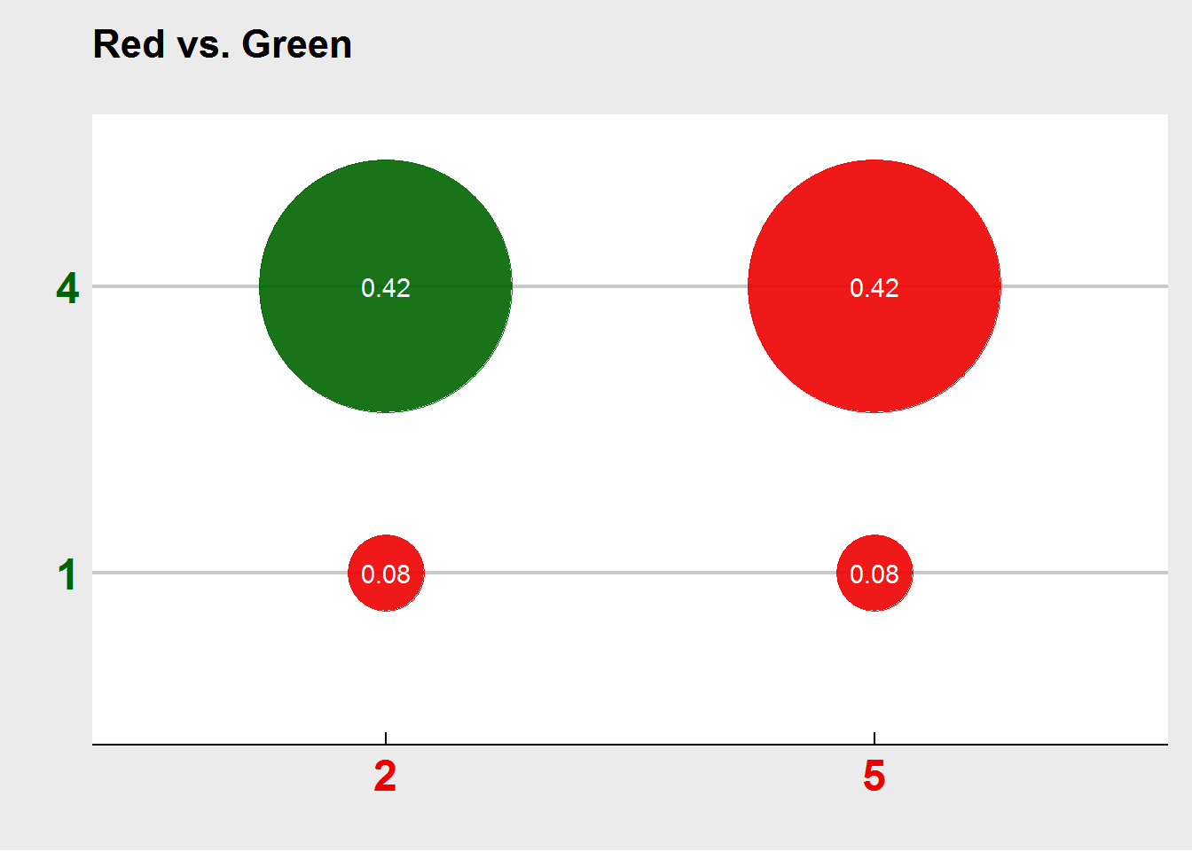
But let’s compare how the red one does against the green one (that previously defeated the blue one). It turns out that the red one now has a slight edge against the green one. The edge is as big as in the previous case, but smaller than in the first scenario. And there we have it, the non-transitive nature of the three dices. If somebody wanted to play a game of dice with you in which the highest number wins, and you would have to pick a die first, you would ultimately always lose, because whatever die you pick, your opponent can pick one that will beat it in the long run.
Finally, let’s consider a different type of game. Instead of two players, we have three players, who all roll their die at the same time, and the highest roll wins. We now need to consider three (independent) events happening. For example, the green die coming up 5 (\(1/2\)), the red one coming up 1 (\(1/6\)), and the blue one coming up 6 (\(1/6\)). The joint probability of this happening is just the product of all three probabilities, which in this case is about 1%. If we do this for all possible 8 outcomes, we get the following plot.
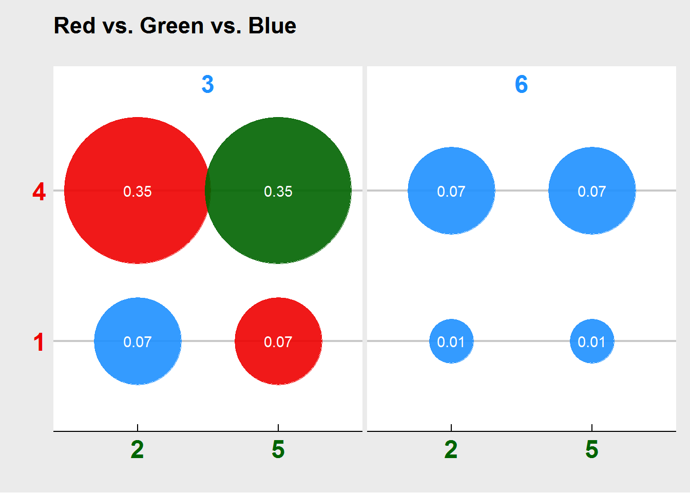
And here we see that the red die is in fact the best of all three dice with an average probability of winning of around 42%. Compared with the blue one which has a dismal 23%, and the green one with 35%. In the game with two players, it pays to be the last to pick a die, but in the game with three players, it’s beneficial to be the first to pick - in this case pick the red one.
library(plyr)
library(broom)
library(ggplot2)
library(ggthemes)
library(magrittr)
library(dplyr)
library(tidyr)

dices <- function() {
  blue <- sample(c(3,3,3,3,3,6),1)
  red <- sample(c(4,4,4,4,4,1),1)
  green <- sample(c(2,2,2,5,5,5),1)
  d <- c(blue,green,red)
  return(d)
}


res <- data.frame(raply(100000,dices))
names(res) <- c("blue","red","green")


round(prop.table(table(res$blue)),2) %>% tidy() %>%
ggplot() +  geom_bar(aes(weight=Freq, x=Var1),fill="dodgerblue",alpha=.9) + ggtitle("Blue\n") +
  xlab("") + ylab("") +
  theme_economist_white() +
  theme(axis.text.x = element_text(face="bold", color="dodgerblue",size=18),
        axis.text.y = element_text(size=12))

round(prop.table(table(res$gree)),2) %>% tidy() %>%
  ggplot() +  geom_bar(aes(weight=Freq, x=Var1),fill="darkgreen",alpha=.9) + ggtitle("Green\n") +
  xlab("") + ylab("") +
  theme_economist_white() +
  theme(axis.text.x = element_text(face="bold", color="darkgreen",size=18),
        axis.text.y = element_text(size=12))

round(prop.table(table(res$red)),2) %>% tidy() %>%
  ggplot() +  geom_bar(aes(weight=Freq, x=Var1),fill="red2",alpha=.9) + ggtitle("Red\n") +
  xlab("") + ylab("") +
  theme_economist_white() +
  theme(axis.text.x = element_text(face="bold", color="red2",size=18),
        axis.text.y = element_text(size=12))


round(prop.table(table(res$blue,res$green)),2) %>% tidy() %>%
ggplot(aes(Var1, Var2)) +
  geom_point(aes(size = Freq), alpha=.9, color=c("dodgerblue","dodgerblue","darkgreen","dodgerblue"), show.legend=FALSE) +
  geom_text(aes(label = Freq), color="white") +
  scale_size(range = c(15,50)) + ggtitle("Blue vs. Green\n") +
  xlab("") + ylab("") +
  theme_economist_white()+
  theme(axis.text.x = element_text(face="bold", color="dodgerblue",size=18),
        axis.text.y = element_text(face="bold", color="darkgreen",size=18))


round(prop.table(table(res$blue,res$red)),2) %>% tidy() %>%
  ggplot(aes(Var1, Var2)) +
  geom_point(aes(size = Freq), alpha=0.9, color=c("dodgerblue","dodgerblue","red2","dodgerblue"), show.legend=FALSE) +
  geom_text(aes(label = Freq), color="white") +
  scale_size(range = c(15,50)) + ggtitle("Blue vs. Red\n") +
  xlab("") + ylab("") +
  theme_economist_white()+
  theme(axis.text.x = element_text(face="bold", color="dodgerblue",size=18),
        axis.text.y = element_text(face="bold", color="red2",size=18))


round(prop.table(table(res$red,res$green)),2) %>% tidy() %>%
  ggplot(aes(Var1, Var2)) +
  geom_point(aes(size = Freq), alpha=0.9, color=c("red2","red2","darkgreen","red2"), show.legend=FALSE) +
  geom_text(aes(label = Freq), color="white") +
  scale_size(range = c(15,50)) + ggtitle("Red vs. Green\n") +
  xlab("") + ylab("") +
  theme_economist_white()+
  theme(axis.text.x = element_text(face="bold", color="red2",size=18),
        axis.text.y = element_text(face="bold", color="darkgreen",size=18))


round(prop.table(table(res$red,res$green,res$blue)),2) %>% tidy() %>%
  ggplot(aes(Var1, Var2)) +
  geom_point(aes(size = Freq), alpha=0.9, color=c("dodgerblue","red2","darkgreen","red2","dodgerblue","dodgerblue","dodgerblue","dodgerblue"), show.legend=FALSE) +
  geom_text(aes(label = Freq), color="white") +
  scale_size(range = c(15,50)) + ggtitle("Red vs. Green vs. Blue\n") +
  xlab("") + ylab("") +
  theme_economist_white()+
  theme(axis.text.x = element_text(face="bold", color="darkgreen",size=18),
        axis.text.y = element_text(face="bold", color="red2",size=18)) +
  facet_wrap(~Var3) +
  theme(strip.text = element_text(color = 'dodgerblue',face="bold",size=18))