
Felix Thoemmes


Inspired by a recent discussion on SEMNET, I decided to publish a short blog post about the front-door criterion. The front-door criterion was developed by Judea Pearl, as a means to identify and estimate a causal effect in the presence of unobserved confounders.
Consider the following DAG (directed acyclical graph) in which a treatment X has an effect on an outcome Y. This effect however cannot directly be estimated without bias, because there is an unobserved confounder U. However, there is a variable M that is caused by X, and causes Y, and importantly is not itself caused by the unobserved confounder U.
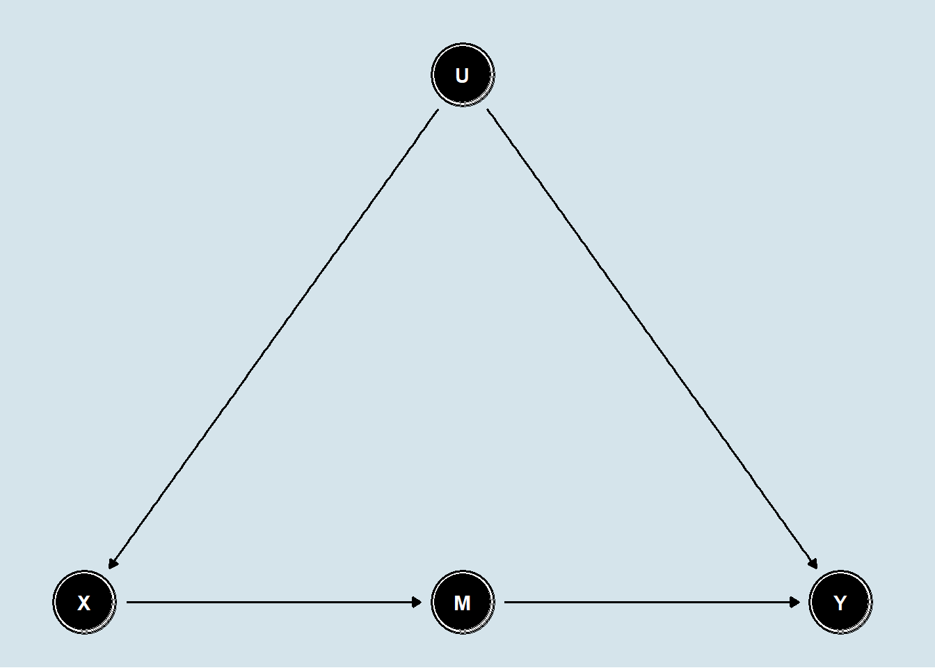
Equally important is that the effect of X on Y goes entirely through M. Psychologists would tend to call this a full mediation model. For a fuller description of the front-door criterion, you can check Pearl’s book “Causality”, but here is a brief intuitive explanation.
The total effect of X on Y, can be decomposed into the effects of X on M, and M on Y. The effect of X on M can be estimated without bias, because there is no open back-door path - the only back-door path that goes through U is blocked by the collider Y. The effect of M on Y can also be estimated without bias, because there is only one open back-door path via U, but we can close it by conditioning on X. Once we can estimate these two effects, we can use them to construct the total effect. In parametric, linear models, the total effect of X on Y, will just be the product of the two paths. Again, we see the parallels to classic mediation analysis - this is how one typically computes the the indirect effect in mediation models.
In the following example, I want to demonstrate the front-door criterion using parametric, linear models. I will use a SEM (structural equation model) and ML estimation to compute the total effect of X on Y.
The data-generating model mirrors the DAG in Figure 1, and can be described as follows:
\(U \sim N(0,1)\)
\(X = .5*U + \epsilon_X\)
\(M = .5*X + \epsilon_M\)
\(Y = .5*M + .5*U + \epsilon_Y\)
\(\epsilon_X, \epsilon_M, \epsilon_Y \sim N(0,1)\)
The true total effect of X on Y in this data-generating model is .25.
I will simulate data from this model, and estimate (a) an unadjusted treatment effect of X on Y, (b) a front-door adjusted treatment effect of X on Y, and (c) for comparative purposes an adjusted treatment effect of X on Y, assuming that we have access to the unobserved confounder U.
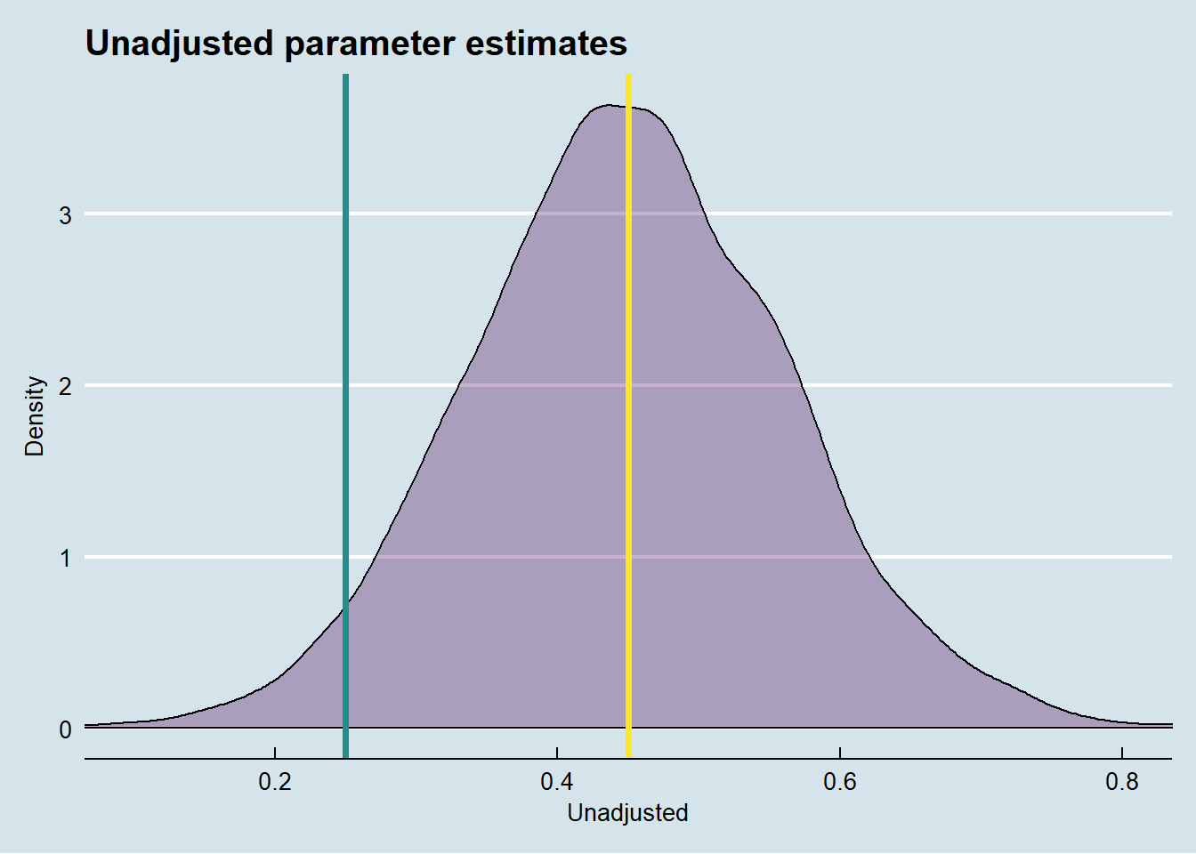
As we can see, the unadjusted treatment effect is biased - and badly so. We would expect this, given the presence of the unobserved confounder U. Now let’s see how the front-door adjusted treatment effect fares.
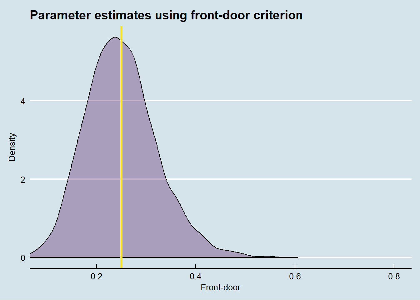
As we can see in the graph above, it is generally unbiased. The two lines which represent the true treatment effect (.25) and the average of the estimated front-door effects are essentially on top of each other. The remarkable thing about the front-door adjusted treatment effect is that we can obtain unbiased estimate, despite the fact that we do NOT have observed the confounder.
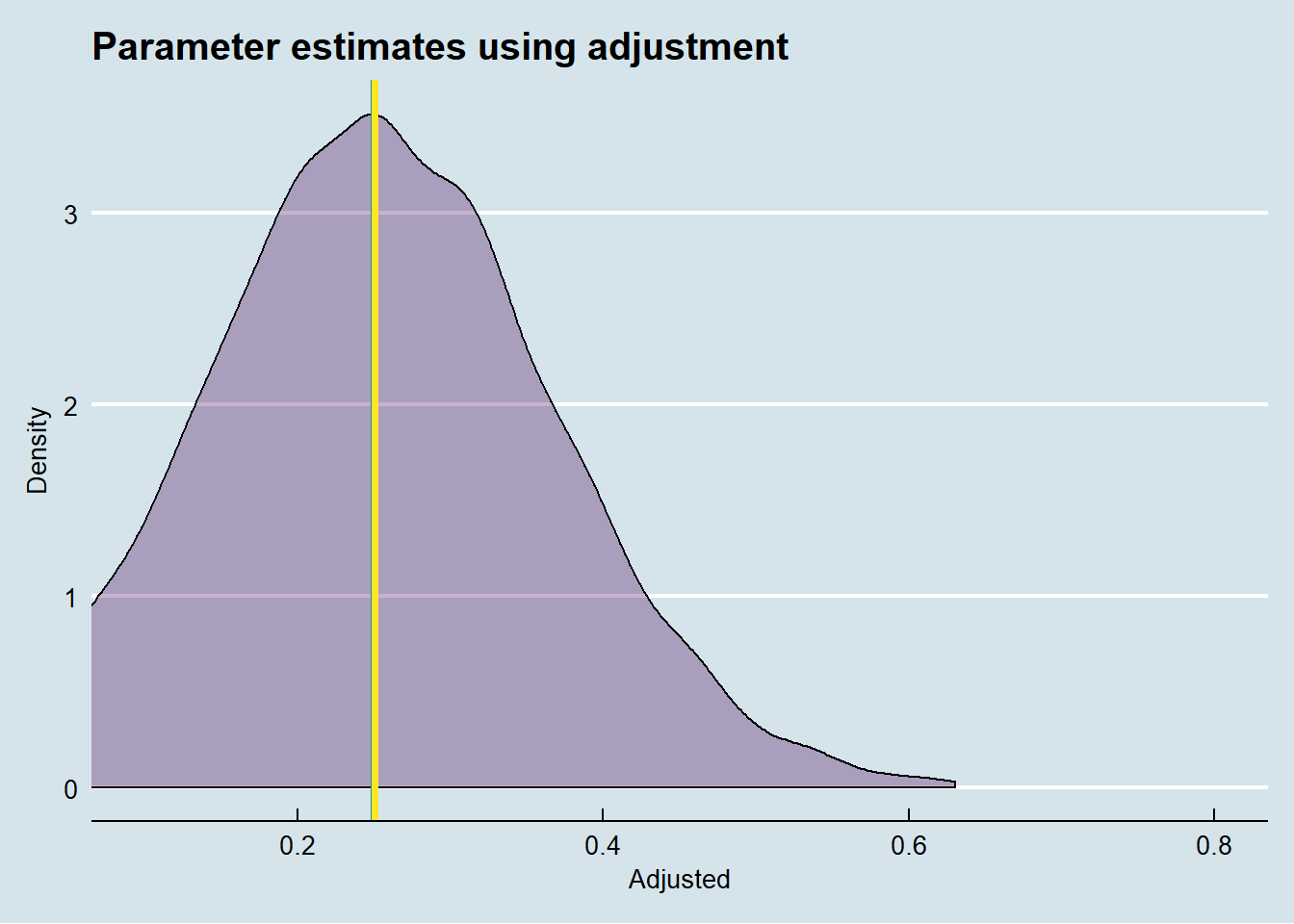
Just for comparative purposes, here are the treatment effects that we derive from using regression adjustment, and pretending that we have access to the unobserved confounder. This effect is of course also unbiased.
Just like instrumental variable estimation, the front-door criterion allows us to obtain unbiased treatment effects, without the need of having to collect all unobserved confouders. This however, does not mean that using the front-door criterion is easy, in a sense that it could be routinely done. The hard part is finding a variable M that fulfills the requirements of (a) being “shielded” off the unobserved confounders of X and Y (via X), and (b) the absence of a direct effect of X on Y.
I am personally not aware of many published examples of the front-door criterion. Alex Chino has a much more extensive blog post, where he discusses the example of voting patterns, same school background, and seating assignment in the US Senate published by Cohen and Malloy (2010) (http://www.nber.org/papers/w16437). Overall, I think it’s fair to say that variables that would permit one to use the front-door criterion are rare - in the same sense that instrumental variables tend to be somewhat rare. Or maybe we just haven’t looked for them very hard, as the front-door criterion is still not widely known.
library(lavaan)
library(ggplot2)
library(ggthemes)
library(ggdag)
library(dagitty)


x <- dagitty('dag {
             bb="0,0,1,1"
             M [pos="0.5,0"]
             U [pos="0.5,0.5"]
             X [pos="0,0"]
             Y [pos="1,0"]
             M -> Y
             U -> X
             U -> Y
             X -> M
             }')

ggdag(x) + theme_economist() + theme(axis.line=element_blank(),axis.text.x=element_blank(),
                                     axis.text.y=element_blank(),axis.ticks=element_blank(),
                                     axis.title.x=element_blank(),
                                     axis.title.y=element_blank(),legend.position="none",
                                     panel.background=element_blank(),panel.border=element_blank(),panel.grid.major=element_blank())


fd <- function(n,a,b,u1,u2) {
  U <- rnorm(n,0,1)
  e_x <- rnorm(n,0,1)
  e_m <- rnorm(n,0,1)
  e_y <- rnorm(n,0,1)
  X <- u1*U + e_x
  M <- a*X + e_m
  Y <- b*M + u2*U + e_y

  df1 <- data.frame(X,M,Y,U)

  fdmodel <- "M ~ a*X
              Y ~ b*M
              X ~~ Y
              FD := a*b"


  fd <- sem(fdmodel,df1)@ParTable$est[7]
  unadj <- coef(lm(Y~X))[2]
  adj <- coef(lm(Y~X+U))[2]
  return(c(fd,unadj,adj))
}

res <- data.frame(t(replicate(5000,fd(100,.5,.5,.5,.5))))
names(res) <- c("fd","unadj","adj")

cols <- viridis(3)

ggplot(res,aes(x=fd)) + geom_density(alpha=.3,fill=cols[1]) + theme_economist() +
  geom_vline(xintercept = .25,col=cols[2],size=1.25) +
  geom_vline(xintercept = mean(res$fd),col=cols[3],size=1.25) + xlab("Front-door") + ylab("Density") +
  coord_cartesian(xlim=c(.1,.8)) + ggtitle("Parameter estimates using front-door criterion")

ggplot(res,aes(x=adj)) + geom_density(alpha=.3,fill=cols[1]) + theme_economist() +
  geom_vline(xintercept = .25,col=cols[2],size=1.25) +
  geom_vline(xintercept = mean(res$adj),col=cols[3],size=1.25) + xlab("Adjusted") + ylab("Density") +
  coord_cartesian(xlim=c(.1,.8)) + ggtitle("Parameter estimates using adjustment")

ggplot(res,aes(x=unadj)) + geom_density(alpha=.3,fill=cols[1]) + theme_economist() +
  geom_vline(xintercept = .25,col=cols[2],size=1.25) +
  geom_vline(xintercept = mean(res$unadj),col=cols[3],size=1.25) + xlab("Unadjusted") + ylab("Density") +
  coord_cartesian(xlim=c(.1,.8)) + ggtitle("Unadjusted parameter estimates")